贝叶斯推断的自动批处理#
![]()

此笔记本演示了一个简单的贝叶斯推断示例,其中自动批处理使编写用户代码更容易、更易于阅读,并且更不容易包含错误。
灵感来自 @davmre 的笔记本。
import matplotlib.pyplot as plt

import jax

import jax.numpy as jnp
import jax.scipy as jsp
from jax import random

import numpy as np
import scipy as sp
生成一个虚假的二元分类数据集#
np.random.seed(10009)

num_features = 10
num_points = 100

true_beta = np.random.randn(num_features).astype(jnp.float32)
all_x = np.random.randn(num_points, num_features).astype(jnp.float32)
y = (np.random.rand(num_points) < sp.special.expit(all_x.dot(true_beta))).astype(jnp.int32)
y
array([0, 0, 0, 1, 1, 1, 0, 1, 1, 1, 1, 1, 0, 1, 0, 0, 0, 1, 1, 1, 1, 0,
       1, 0, 0, 0, 0, 0, 1, 0, 1, 0, 0, 0, 1, 0, 0, 0, 1, 0, 0, 0, 0, 0,
       1, 1, 0, 1, 0, 0, 0, 1, 1, 0, 0, 1, 0, 0, 0, 0, 0, 1, 1, 0, 0, 0,
       0, 1, 1, 0, 0, 0, 1, 1, 1, 1, 1, 1, 0, 0, 0, 1, 1, 0, 1, 0, 1, 1,
       1, 0, 1, 0, 0, 0, 0, 1, 0, 1, 0, 0], dtype=int32)
为模型编写对数联合函数#
我们将编写一个非批处理版本,一个手动批处理版本,以及一个自动批处理版本。
非批处理#
def log_joint(beta):
    result = 0.
    # Note that no `axis` parameter is provided to `jnp.sum`.
    result = result + jnp.sum(jsp.stats.norm.logpdf(beta, loc=0., scale=1.))
    result = result + jnp.sum(-jnp.log(1 + jnp.exp(-(2*y-1) * jnp.dot(all_x, beta))))
    return result
log_joint(np.random.randn(num_features))
Array(-213.2356, dtype=float32)
# This doesn't work, because we didn't write `log_prob()` to handle batching.
try:
  batch_size = 10
  batched_test_beta = np.random.randn(batch_size, num_features)

  log_joint(np.random.randn(batch_size, num_features))
except ValueError as e:
  print("Caught expected exception " + str(e))
Caught expected exception Incompatible shapes for broadcasting: shapes=[(100,), (100, 10)]
手动批处理#
def batched_log_joint(beta):
    result = 0.
    # Here (and below) `sum` needs an `axis` parameter. At best, forgetting to set axis
    # or setting it incorrectly yields an error; at worst, it silently changes the
    # semantics of the model.
    result = result + jnp.sum(jsp.stats.norm.logpdf(beta, loc=0., scale=1.),
                           axis=-1)
    # Note the multiple transposes. Getting this right is not rocket science,
    # but it's also not totally mindless. (I didn't get it right on the first
    # try.)
    result = result + jnp.sum(-jnp.log(1 + jnp.exp(-(2*y-1) * jnp.dot(all_x, beta.T).T)),
                           axis=-1)
    return result
batch_size = 10
batched_test_beta = np.random.randn(batch_size, num_features)

batched_log_joint(batched_test_beta)
Array([-147.84033 , -207.02205 , -109.26075 , -243.80833 , -163.0291  ,
       -143.84848 , -160.28773 , -113.771706, -126.60544 , -190.81992 ],      dtype=float32)
使用 vmap 自动批处理#
它能正常工作。
vmap_batched_log_joint = jax.vmap(log_joint)
vmap_batched_log_joint(batched_test_beta)
Array([-147.84033 , -207.02205 , -109.26075 , -243.80833 , -163.0291  ,
       -143.84848 , -160.28773 , -113.771706, -126.60544 , -190.81992 ],      dtype=float32)
自包含的变分推断示例#
一些代码是从上面复制的。
设置(批处理的)对数联合函数#
@jax.jit
def log_joint(beta):
    result = 0.
    # Note that no `axis` parameter is provided to `jnp.sum`.
    result = result + jnp.sum(jsp.stats.norm.logpdf(beta, loc=0., scale=10.))
    result = result + jnp.sum(-jnp.log(1 + jnp.exp(-(2*y-1) * jnp.dot(all_x, beta))))
    return result

batched_log_joint = jax.jit(jax.vmap(log_joint))
定义 ELBO 及其梯度#
def elbo(beta_loc, beta_log_scale, epsilon):
    beta_sample = beta_loc + jnp.exp(beta_log_scale) * epsilon
    return jnp.mean(batched_log_joint(beta_sample), 0) + jnp.sum(beta_log_scale - 0.5 * np.log(2*np.pi))

elbo = jax.jit(elbo)
elbo_val_and_grad = jax.jit(jax.value_and_grad(elbo, argnums=(0, 1)))
使用 SGD 优化 ELBO#
def normal_sample(key, shape):
    """Convenience function for quasi-stateful RNG."""
    new_key, sub_key = random.split(key)
    return new_key, random.normal(sub_key, shape)

normal_sample = jax.jit(normal_sample, static_argnums=(1,))

key = random.key(10003)

beta_loc = jnp.zeros(num_features, jnp.float32)
beta_log_scale = jnp.zeros(num_features, jnp.float32)

step_size = 0.01
batch_size = 128
epsilon_shape = (batch_size, num_features)
for i in range(1000):
    key, epsilon = normal_sample(key, epsilon_shape)
    elbo_val, (beta_loc_grad, beta_log_scale_grad) = elbo_val_and_grad(
        beta_loc, beta_log_scale, epsilon)
    beta_loc += step_size * beta_loc_grad
    beta_log_scale += step_size * beta_log_scale_grad
    if i % 10 == 0:
        print('{}\t{}'.format(i, elbo_val))
0	-175.56158447265625
10	-112.76364135742188
20	-102.41358947753906
30	-100.27794647216797
40	-99.55817413330078
50	-98.17999267578125
60	-98.60237884521484
70	-97.69735717773438
80	-97.5322494506836
90	-97.17939758300781
100	-97.09413146972656
110	-97.40316772460938
120	-97.0446548461914
130	-97.20582580566406
140	-96.8903579711914
150	-96.91873931884766
160	-97.00558471679688
170	-97.45591735839844
180	-96.73573303222656
190	-96.95585632324219
200	-97.51350402832031
210	-96.92330932617188
220	-97.03158569335938
230	-96.88632202148438
240	-96.96971130371094
250	-97.35342407226562
260	-97.07598876953125
270	-97.24359893798828
280	-97.23466491699219
290	-97.02442932128906
300	-97.00311279296875
310	-97.07693481445312
320	-97.3313980102539
330	-97.15113830566406
340	-97.28958129882812
350	-97.41973114013672
360	-96.95799255371094
370	-97.36981201171875
380	-97.00273132324219
390	-97.10066986083984
400	-97.13655090332031
410	-96.87237548828125
420	-97.2408447265625
430	-97.04019165039062
440	-96.68864440917969
450	-97.19795989990234
460	-97.18959045410156
470	-97.09815979003906
480	-97.11341857910156
490	-97.20773315429688
500	-97.39350128173828
510	-97.25328063964844
520	-97.20199584960938
530	-96.95065307617188
540	-97.37591552734375
550	-96.98526763916016
560	-97.01451873779297
570	-96.9732894897461
580	-97.04314422607422
590	-97.38459777832031
600	-97.31582641601562
610	-97.10185241699219
620	-97.22990417480469
630	-97.18515014648438
640	-97.15637969970703
650	-97.13623046875
660	-97.0641860961914
670	-97.17774200439453
680	-97.31779479980469
690	-97.4280776977539
700	-97.18154907226562
710	-97.57279968261719
720	-96.99563598632812
730	-97.15852355957031
740	-96.85629272460938
750	-96.89025115966797
760	-97.11228942871094
770	-97.21411895751953
780	-96.99479675292969
790	-97.30390930175781
800	-96.98690795898438
810	-97.12832641601562
820	-97.51512145996094
830	-97.4146728515625
840	-96.89872741699219
850	-96.84567260742188
860	-97.2318344116211
870	-97.24137115478516
880	-96.74853515625
890	-97.09489440917969
900	-97.138671875
910	-96.79051208496094
920	-97.06620788574219
930	-97.14911651611328
940	-97.26902770996094
950	-97.0196533203125
960	-96.95348358154297
970	-97.13890838623047
980	-97.60130310058594
990	-97.2507553100586
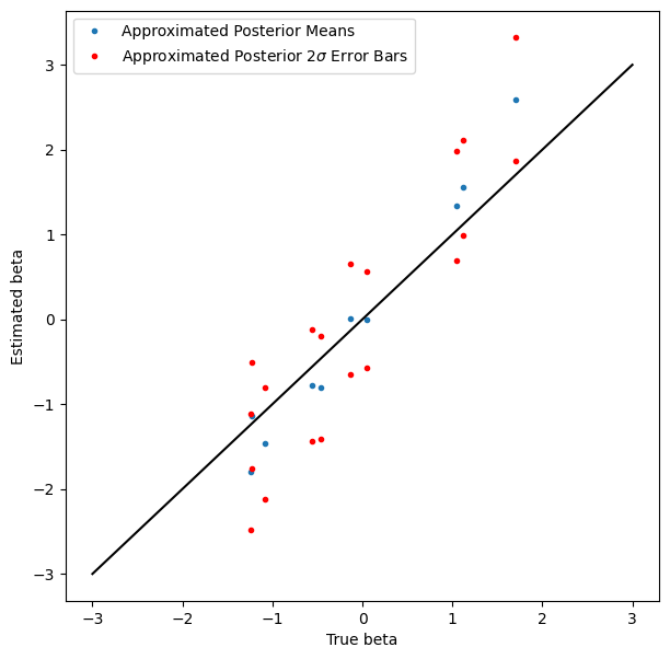
显示结果#
覆盖率可能不如我们希望的那么好,但还不错,而且没人说变分推断是精确的。
plt.figure(figsize=(7, 7))
plt.plot(true_beta, beta_loc, '.', label='Approximated Posterior Means')
plt.plot(true_beta, beta_loc + 2*jnp.exp(beta_log_scale), 'r.', label=r'Approximated Posterior $2\sigma$ Error Bars')
plt.plot(true_beta, beta_loc - 2*jnp.exp(beta_log_scale), 'r.')
plot_scale = 3
plt.plot([-plot_scale, plot_scale], [-plot_scale, plot_scale], 'k')
plt.xlabel('True beta')
plt.ylabel('Estimated beta')
plt.legend(loc='best')
<matplotlib.legend.Legend at 0x7f667d8fb460>